Orthogonal packing of rectangles
within isotropic convex regions

This Web site provides additional material to the paper

E. G. Birgin and R. D. Lobato. Orthogonal packing of identical rectangles within isotropic convex regions. Computers & Industrial Engineering (2010) 59, 595–602.

The full text is locally available in PDF and PS formats. The full text can also be found at ScienceDirect. The computer implementation in Fortran 77/95 is available to download under the terms of the GNU General Public License. Below you can find instructions on how to compile and run the program, visualize the solution, and modify the program in order to solve your own instance of the problem. If you have any questions, please send an e-mail to rafael@lobato.it.

Compiling and running it

To compile the program, just type

./compile.sh

To run it, type

./igenpack

The program will ask you which problem you would like to solve (choose a number between 1 and 16 to solve one of the 16 problems presented in the paper) and the minimum and maximum number of rectangles the method will try to pack.

The program will output the number of rectangles that have been packed until the upper bound is reached.

Graphical representation of the solution

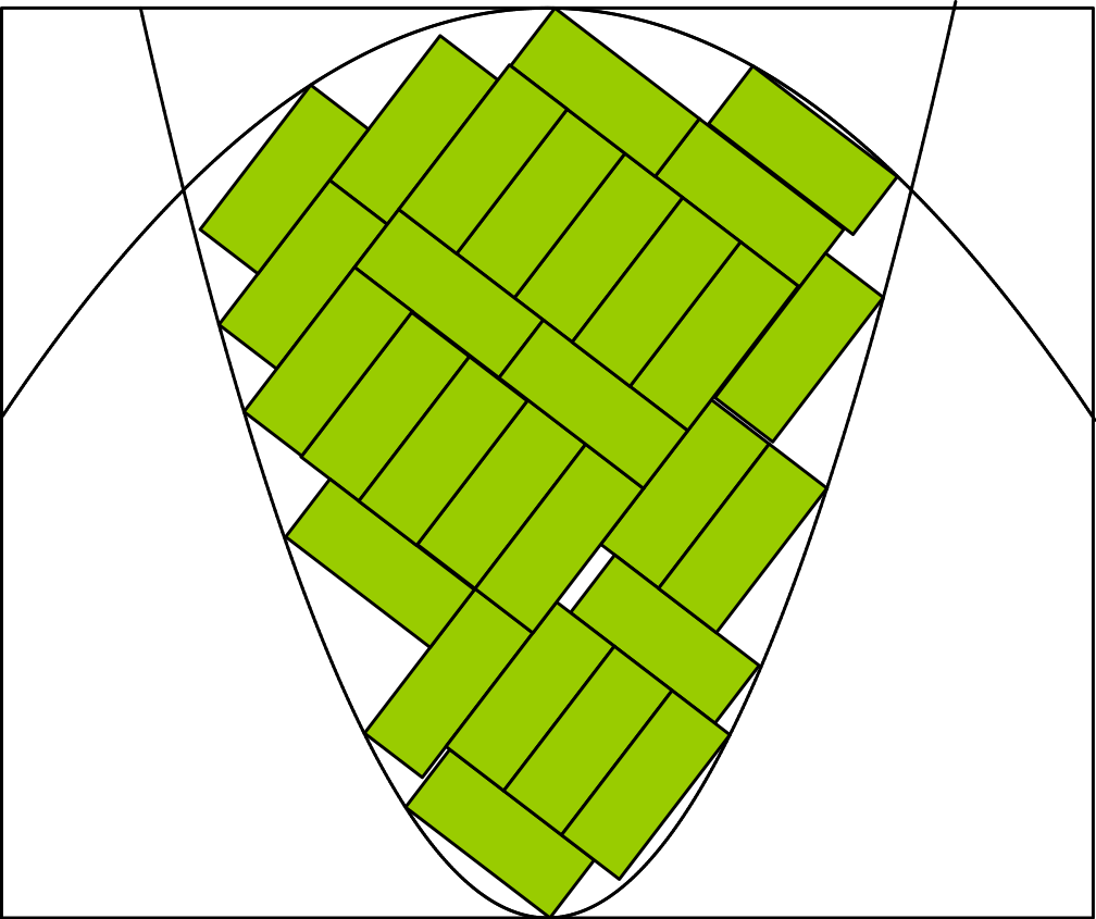
To generate the graphical representation of the solution, first compile the MetaPost file solution.mp, which was created by IAlgencan, by typing

mpost solution.mp

It will generate a file called solution.1. Then, to create a PostScript file, just type

latex solution.tex

and then

dvips solution.dvi -o solution.ps

The PostScript file with the graphical representation of the solution will be in the file called solution.ps. To see this file, type, for example,

gv solution.ps

Solving your own problem

To solve your own instance of the problem, you just need a basic knowledge of Fortran 77/95 programming language to edit the file Packing.f95. In this file you will need add the information of your problem in the following subroutines:

• DEFPRO is the subroutine that defines some information of the problem.

  Rectangular item information

  dx: half of the horizontal side of the rectangles
  dy: half of the vertical side of the rectangles

  Box constraints of the convex region

  lx: lower bound for the x-axis
  ux: upper bound for the x-axis
  ly: lower bound for the y-axis
  uy: upper bound for the y-axis

  Extra-information of the convex region

  The following four parameters must represent a limited box that contains the convex region. See, for example, problems 4, 5, 6 and 11 that have their boxes (which are not part of the definition of the convex region) drawn in Figure 2 of the paper. You can see that these boxes do not take part in the definition of the convex regions in Table 1 of the paper.

  xmin: containing-box lower bound for the x-axis
  xmax: containing-box upper bound for the y-axis
  ymin: containing-box lower bound for the x-axis
  ymax: containing-box upper bound for the y-axis

  More information of the convex region

  r: number of smooth functions in the definition of the convex region

• EVALW is the subroutine that implements the smooth functions that define the convex region.

• EVALDW is the subroutine that computes the derivatives of the smooth functions that define the convex region.

• DRAWSOL is the subroutine that draws the graphical representation of the solution. The piece of code that draws the packed items is common to all the problems and you do not need to modify it. You just need to add the piece of code that draws the convex region. If you are not interested in the graphical representation of the solution, you may skip this subroutine.

After having modified the four subroutines, just compile the program and run it as explained above.

Sponsor

This work was partially supported by the Brazilian agency FAPESP (Fundação de Amparo à Pesquisa do Estado de São Paulo).